Fuzzy Logic Enhanced Neural Network Update Rule Derivation
for training FLENNs
Introduction
This discussion builds on the introductions to NNs and FLENNs.The simple idea of fuzzy-logic-enhanced neural networks is to add fuzzy-logic nodes within NN layers. The outputs of these nodes are fuzzy-logical, or may I simply say, logical, combinations of their inputs.
To wit: for some or all nodes or node pairs in a given NN level \(l\), we may add logical nodes to the layer in a FL-enhanced node set \(l^{?!}\) each carrying out some logical operation on its input(s), along with weighted links from them to nodes in the next layer. The designer may choose more or fewer logic nodes and more or fewer successor links to add to the network; indeed, we do not assume \(l^{?!}\ne \emptyset\); so this model reduces to regular NNs in that case.With so much structure shared, please forgive the occasional redundancy between this discussion and that of regular NNs and their training in these pages.
Here our purpose is mathematical description of FLENNs including their feedforward operation as well as backpropagation for training, and in particular we will seek to apply successive linear approximation (a.k.a. "Newton Raphson") in the update rule for fuzzy logic enhanced neural network training.
As explained here, SLA is that special case of gradient descent (\(\large \hat w = w - \delta e'\)) which specifies \(\delta = \frac{1}{e''}\).
Terms
Let's establish terms, notation, conventions, and intermediate constructs, so we can describe this cleanly.See the side bar for several which apply to regular NNs: Weights \(W\), sum of weighted inputs \(s\), threshold function \(\theta\), node outputs \(o\), error \(e\), its derivative \(e'\) and chain rule components of \(e'\) namely \(A,B\).
In FLENNs as with regular NNs, the intermediate values \(o, A, B\), etc., are recursively calculated based on the local network architecture, i.e., via node connections and rules of value transmissions. FLENNs add some extra nodes and connections, and for those nodes there are different rules by which values are transmitted.
In addition to the graphical conventions taught here we add the generic Fuzzy Logic Node graphical convention as follows:
Each poses a question (?), then provides the answer (!) with definiteness and clarity, thus ? then !.The "?! functions" are as follows (a relabelling of this).
| name | symbol | ?! function |
| NOT | ¬ o1 | NOT\((o1)=(1-o_1)\) |
| AND | o1∧o2 | AND\((o_1,o_2)=\) min(\(o_1,o_2\)) |
| OR | o1∨o2 | OR\((o_1,o_2)=\) max\((o_1,o_2)\) |
| XOR | o1⊻o2 | XOR\((o_1,o_2) = \frac{1}{2}(|o_1-o_2|+1-|o_1+o_2-1|)\) |
| IMPLIES | o1→o2 or o2 ∨ ¬ o1 | IMPLIES\((o_1,o_2) = \) max (\(1-o_1,o_2\)) |
An NN layer may be referred to by its number, such as \(l\), as context allows, and subcategorized with diacritics as follows:
- Let \(l' = l\ \)∪\(\ l^{?!}\) refer to a fuzzy-logic enhanced layer as a whole,
- where \(l\) refers to the set of all the regular NN nodes in the layer, exclusive of logic nodes, and
- where \(l^{?!}\) refers to the set of all and only the fuzzy-logic nodes added to the layer.
From the perspective of the following layer \(l+1\), the links from layer "\(l\)" come from any of the nodes in \(l'\): some from nodes in \(l\) and some from nodes in \(l^{?!}\).
Feed Forward
We start with the feedforward calculations proceeding from the inputs to the output.
- Base case: Layer 0=0' holds in its nodes all the system inputs,
which are made available to the next layer as the outputs of
layer 0'.
- Recursion:
- Multiply-Add: As with regular NNs, multiply outputs of the previous layer \((l-1)'\) by their link weights to the regular (non-logic) nodes of the current layer \(l\).
- That is, for each node \(j\ \) ∈ \(\ l\) the sum of link-weighted
outputs from layer \((l-1)'\) becomes the value \(s_j\) as in
the regular case:
\(s_j = \sum_{i\in (l-1)'} w_{ij} o_i \)
- Threshold: Given \(s_j\) apply the threshold function
to it yielding the node output \(o_j\) (see sidebar \(\theta\)).
\(o_j = \theta(s_j)\)
- Apply Logic
For each node \(j^{?!}\) in \(l^{?!}\), calculate its output
from its input(s) using the applicable ?! function or logic rule.
(We assume we know what feeds \(j^{?!}\), and which ?! rule it uses.) - Exit if Done otherwise Recurse, incrementing l to l+1.
Repeating until done (\(l=N\)), we build up the outputs for all nodes, regular and logical, in the entire network, and of course that includes the final output value \(\hat z\) which the network predicts for the inputs it was given.
So much for the forward process, used in classification or practical operation. The output(s) could be the answer to a classification question, such as "Does this picture contain a cat?", or could be a vector such as an automatic-driving vector of vehicle controls. But the performance of such systems is only as good as their training.
Back Propagation
Now the backward process is needed, to find the derivatives of the errors with respect to the parameters of the model. At each point we will make use of a certain linearity, namely that at a given node, the derivative of a sum of outputs is the sum of the derivatives of the outputs:
\(d\sum = \sum d\)
This is easy in the case of regular neural networks since each node output lives exclusively on a single node in the network.
But in the case of logic nodes, in a data-dependent way, the node output might also live on a following logic node. For example, if \(o_3 = \ \)AND\((o_1,o_2) = \ \)min\((o_1,o_2)\), then depending on \(o_2, o_3\) might have the value of \(o_1\), so that now \(o_1\) isn't just the output of node 1, it is also the output of node 3. In that case, when we add up the chain rule derivatives on all the paths coming back to node 1 with last value \(o_1\), we must also add the other paths which have the value \(o_1\), which may include the logical outputs that happen to include \(o_1\). We will carefully construct the equations and process for this below.
Since the totality of nodes in a layer \(l'\) comprise two subsets, \(l\) and \(l^{?!}\), and the latter are fed from the former, there are therefore three classes of links from a given layer:
- 1) those from nodes in \(l\) to nodes in \((l+1)\),
- 2) those from nodes in \(l\) to nodes in \(l^{?!}\),
- 3) those from nodes in \(l^{?!}\) to nodes in \((l+1)\),
The backward recursion begins with the error \(e=\frac{1}{2}(\hat z-z)^2\), and \(\frac{de}{d\hat z} = \hat z - z\) and \(\frac{d^2e}{(d\hat z)^2}=1\), same as in the regular NN case (see sidebar). \(\hat z\) is another name for \(o_z\) which is the scalar or vector-valued output for node(s) \(z\) ∈ \(l_{final}\). This gives us the base case for a recursive construction continuing from the final layer one layer at a time to the input layer \(l_{0}\).
To define \(A, B, C, D, e, o_z, \hat z\), it will help to have a schematic drawing of the local neighborhood of a regular and a logical node.
To keep things readable, each node, link, and layer in the schematic represents a set of others like it. Thus one instance, a box labelled \(j^{?!}\), represents all the logic nodes in layer \(l^{?!}\), which is the fuzzy-logic-enhanced part of layer \(l'\). The equations will indicate how we generalize over all the nodes, links, and layers.
Note that the inputs for logic nodes are not summed (in the drawing, the links to the ?! node are shown without the arrowheads that would indicate summation). Instead they are taken directly (or what amounts to the same, weighted by 1.0) from a predecessor's output value into one of its inputs. ?! being a general category, we will wave hands saying, Calculate the output based on whichever ?! function is appropriate to the particular logic node -- and indeed we can assume each logic node knows what it is.
It helps me to move a finger over the drawing while referring to the equations, to make sure my reasoning is valid.
Now, let's define \(A, B, C, D, e, o_z, \hat z\).
| \(o_z=\hat z\) | In case \(k\) is in the final output layer, \(o_k=o_z=\hat z\) is the feedforward final node output, the system output, and the system estimate for \(z\). |
| \(e=\frac{1}{2}(z-\hat z)^2\) | \(e\) is the 'error', the squared difference between target \(z\) and estimate \(\hat z\) |
| \(\large \frac{de}{d\hat z} =\frac{de}{do_z} = \hat z - z\) | Base case for recursive backpropagation |
| \(A_k = \large \frac{de}{do_k}\) | From the base case \((A_z=\frac{de}{do_z})\) or from previous rounds of recursion, we are given \(A_k\) for each \(k\) in \((l+1)\). |
| \(B_k = \large \frac{do_k}{ds_k}\) | \(A_k * B_k\) by the chain rule yields \(\large \frac{de}{ds_k}\). |
| \(C_{jk} = \large \frac{ds_k}{dw_{jk}}\) | \(A_k*B_k * C_{j,k}\) yields \(\large
\frac{de}{dw_{jk}}\) in case of links from regular nodes \(j
\in l\) to \(k \in (l+1)\). Similarly, \(A_k*B_k*C_{j^{?!},k}\) yields \(\large \frac{de}{dw_{j^{?!}k}}\) in case of links from logic nodes \(j^{?!} \in l^{?!}\) to \(k \in (l+1)\).
|
| \(D_{jj^{?!}} = \frac{do_{j^{?!}}}{do_j}\) |
We will also find derivatives across the logic nodes: \(D_{jj^{?!}} =
\frac{do_{j^{?!}}}{do_j}\). D influences the predecessors \(j\) of logical nodes \(j^{?!}\). The total derivative at node \(j\) is the sum of derivatives of \(j\)'s successors which include the weighted links to the next layer \(l+1\) and also the logical input links to the logical nodes \(j^{?!}\) in the logical layer \(l^{?!}\).
|
| \(e'=e'_{jk} = \large \frac{de}{dw_{jk}}\) | This term is the goal of backpropagation. \(e'\) is used in the update rule for \(w_{jk}\), to change it in the right direction. \(A,B,C,D\) will be used in the chain rule recursive decomposition of derivatives so we can get \(e'\) values for not just the final layer but all the way back to the first, eventually training ALL the weights. |
For a given node, or a weight on a link from a given node, the derivative of the errors is the sum of derivatives ...
To calculate the sum of derivatives ...
For a layer \(l+1\) containing nodes \(k\) ∈ \((l+1)\) we are given \(A_k = de/do_k\) and \(A_k' = d^2e/(do_k)^2\). The nodes \(k\) are all those which are visible from the preceding layer \(l'\); none are logic-enhanced nodes.
Dividing \(l'\) into \(l\) and \(l^{?!}\), let's first capture the link-specific derivatives going from \(l^{?!}\) into \((l+1)'\). That will give us everything needed to update the weights from \(l^{?!}\) to \((l+1)' because there is no complexity after the enhanced nodes; none of them go to other logic nodes within the layer, so that forms a completed subset.
Second, we will calculate the derivatives of the weights from all the regular nodes, separately including the successors in \((l+1)\) and separately including the logical successors in \(l^{?!}\). The \((l+1)\) successors get their weights calculated in the normal way, but the successors in the logic-enhanced sublayer within \(l'\) namely \(l^{?!}\) nodes, need their derivatives to contribute to the \(de/do_j\) through the chain rule operating on pathways through the logic nodes. In particular the fuzzy logic equations have derivatives, and those are multiplied through in the chain rule expressions for paths proceeding within a layer from an \(l\) node to an \(l^{?!}\) node.
The FL equation derivatives follow. Unlike nice polynomial functions their derivatives are discontinuous, which causes some extra work, but unlike nice polynomials functions their derivatives are constants, in fact 1, 0, or -1, easy to calculate, after testing which condition applies:
\(D_{jj^{?!}} = \frac{do_{j^{?!}}}{do_j} = ( \)condition\(\ ? 1 : 0 )\ \) or at worstwhere \(j^{?!}\) ∈ \((l+1)\), and \(j,j_1,j_2\) ∈ \(l'\). Specifically:
\(D_{jj^{?!}} ( \)condition1\(\ ? (\)condition2\(\ ? 1 : 0 ) : -1 )\).
- NOT: \(o_{j^{?!}}=\ \)NOT\((o_j) = 1-o_j,\ \ \ \) so
\(\ \ \ \ \ \ \ \ \ D_{jj^{?!}} = \frac{do_j^{?!}}{do_j} = \frac{d}{do_j} (1-o_j) = -1 \) - AND: \(o_{j^{?!}}=\ \)AND\((o_{j_1},o_{j_2}) = \ \)min\((o_{j_1},o_{j_2}) = \Big|^{o_{j_1}>o_{j_2}}\ \ o_{j_2},\ \ \ \ \Big| \)
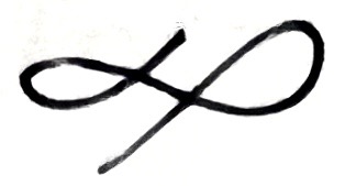 \( o_{j_1},\ \ \ \ \) so
 \(\ \ \ \ \ \ \ \ \ D_{j_1j^{?!}} = \frac{do_{j^{?!}}}{do_{j_1}} = \frac{d}{do_j} \ \)min\((o_{j_1},o_{j_2}) = \ \ \\ \Big|^{o_{j_1}>o_{j_2}}\ \ 0,\ \ \ \ \Big| \)
 \( 1 \)
 - OR: \(o_{j^{?!}}=\ \)OR\((o_{j_1},o_{j_2}) = \ \)max\((o_{j_1},o_{j_2}) = \Big|^{o_{j_1}>o_{j_2}} o_{j_1},\ \ \ \ \Big| \)
 \( \ \ o_{j_2}, \ \ \ \ \) so
 \(\ \ \ \ \ \ \ \ \ D_{j_1j^{?!}} = \frac{do_{j^{?!}}}{do_{j_1}} = \frac{d}{do_j} \ \)max\((o_{j_1},o_{j_2}) = \ \ \\ \Big|^{o_{j_1}>o_{j_2}}\ \ 1,\ \ \ \ \Big| \)
 \( \ \ 0\).
 - IMPLIES: \(o_{j^{?!}}=\ \)IMPLIES\((o_{j_1},o_{j_2}) = \ \)max\((1-o_{j_1},o_{j_2}) = \Big|^{1-o_{j_1}>o_{j_2}}\ \ 1-o_{j_1},\ \ \ \ \Big| \)
 \( o_{j_2}, \ \ \ \ \) so
 \(\ \ \ \ \ \ \ \ \ D_{j_1j^{?!}} = \frac{do_{j^{?!}}}{do_{j_1}} = \frac{d}{do_{j_1}} \ \)max\((1-o_{j_1},o_{j_2}) = \ \ \\ \Big|^{1-o_{j_1}>o_{j_2}} -1,\ \ \ \ \\ \Big| \)
 \( 0,\ \ \ \ \) and
 \(\ \ \ \ \ \ \ \ \ D_{j_2j^{?!}} = \frac{do_{j^{?!}}}{do_{j_2}} = \frac{d}{do_{j_2}} \ \)max\((1-o_{j_1},o_{j_2}) = \ \ \\ \Big|^{1-o_{j_1}>o_{j_2}}\ \ 0,\ \ \ \ \\ \ \ \ \Big| \)
 \(1.\)
 - XOR: Define exhaustive and mutually exclusive conditions \(A, B, C, D\) as follows:
\(A: \ \ \ \ o_{j_1} < o_{j_2},\ \ \ \ o_{j_1} + o_{j_2} \ge 1\)
\(B: \ \ \ \ o_{j_1} \ge o_{j_2},\ \ \ \ o_{j_1} + o_{j_2} \ge 1\)
\(C: \ \ \ \ o_{j_1} \ge o_{j_2},\ \ \ \ o_{j_1} + o_{j_2} < 1\)
\(D: \ \ \ \ o_{j_1} < o_{j_2},\ \ \ \ o_{j_1} + o_{j_2} < 1\)Then \(o_{j^{?!}}=\ \)XOR\((o_{j_1},o_{j_2}) = \frac{1}{2}(|o_{j_1}-o_{j_2}| + 1 - | o_{j_1}+ o_{j_2} - 1 | ) = \)
\(\ \ \ \ \ \ \ \ \ \ \ \ \ \ \ \ \ \ \ \ \ \ \ \ \ \ \ \ \ \ \ \ \ \ \ \ \ \ \ \ \ \ \Big|^A 1-o_{j_1}, \ \ \Big|^B 1-o_{j_2}, \ \ \ \Big|^C o_{j_1}, \ \ \ \ \Big|^D o_{j_2}, \ \ \ \ \) so
\(\ \ \ \ \ \ \ \ \ D_{j_1j^{?!}} = \frac{do_{j^{?!}}}{do_{j_1}} = \ \ \ \ \ \ \Big|^A -1, \ \ \ \ \ \ \ \Big|^B 0, \ \ \ \ \ \ \ \ \ \ \ \ \ \Big|^C 1,\ \ \ \ \ \ \Big|^D 0, \ \ \ \ \ \ \ \) and
\(\ \ \ \ \ \ \ \ \ D_{j_2j^{?!}} = \frac{do_{j^{?!}}}{do_{j_2}} = \ \ \ \ \ \ \Big|^A 0, \ \ \ \ \ \ \ \ \ \ \ \ \Big|^B -1, \ \ \ \ \ \ \ \ \Big|^C 0,\ \ \ \ \ \ \Big|^D 1\).
Thus, evaluated in the various conditions, the derivatives are simply 0,1, or -1: easy.
Just as with nodes \(j\) ∈ \(l\) we will consider nodes \(j^{?!}\) ∈ \(l'\) also as predecessors for each node \(k\) in \((l+1)\). Similar to working backwards toward \(w_{jk}\), where we calculate \(e'_{jk} = \frac{de}{dw_{jk}} = \frac{de}{do_k} \cdot \frac{do_k}{ds_k} \cdot \frac{ds_k}{dw_{jk}} = A_k B_k C_{jk} \), we can do the same to reach the weights \(w_{j_{?!}k}\): \(e'_{j^{?!}k} = \frac{de}{dw_{j^{?!}k}} = \frac{de}{do_k} \cdot \frac{do_k}{ds_k} \cdot \frac{ds_k}{dw_{j^{?!}k}} = A_k B_k C_{j^{?!}k} \). Identically we make use of \(A_k\) given by the base case or previous round of recursion and identically we calculate \(B_k = \frac{ds_k}{do_k} = o_k(1-o_k)\). Then nearly identically we set the value of \(C\) here separately for each \(j^{?!}\) ∈ \(l'\), noting that \(s_k\) is a sum of \(o_{j^{?!}}*w_{j^{?!}k}\) along with outputs from other nodes in \(l'\) multiplied by other weights; taking the derivative with respect to \(w_{j^{?!}k}\) all parts of the sum go to zero except
\(C_{j^{?!}k} = \frac{do_{j^{?!}}*w_{j^{?!}k}}{dw_{j^{?!}k}} = o_{j^{?!}}\).So far then we have the derivatives \(e'_{jk}\) and \(e'_{j^{?!}k}\). Those provide the basis for re-estimating the weights \(w_{jk}\) and \(w_{j^{?!}k}\). But we're not done, we must also propagate back using total derivatives (summing across successors) to calculate first the \(A_{j^{?!}}\)'s and then the \(A_j\)'s for the next layer's weights.
Repeating 25 which applies to nodes \(j^{?!}\) as well as nodes \(j\), we see:
\(A_{j^{?!}} = \large \sum_{k} A_k*B_k*F_{j^{?!}k}\), whereIn these sums \(k\) ranges across all the nodes in the successor layer \(l+1\).
\( \large F_{j^{?!}k} = \frac{\partial s_k}{\partial o_{j^{?!}}} \) \(\large = \frac{\partial}{\partial o_{j^{?!}}} ( \sum_{j'} o_{j'} w_{j',k} ) \) where \(j'\) ∈ \(l'\).
\(\large = \sum_{j'} w_{j,k}|j'=j, \ \ \ \ 0|j'\ne j. \) \(\large = w_{j,k} \)
The whole key is in the next step, which combines the derivatives from all successors of a regular node \(j\) ∈ layer \(l\), which must include both the regular weighted links to nodes \(k\) in the next layer \(l+1\) and the logical links to nodes \(j^{?!}\) in this layer's set of logical nodes, \(l^{?!}\), which are after all, also successors of \(j\). Hence:
\(A_j = \large \sum_{k} A_k*B_k*F_{j^{?!}k} + \sum_{j^{?!}} A_{j^{?!}}*D_{j,j^{?!}}\)
Here the sum over nodes \(j^{?!}\) is over all the logical successors of node \(j\).
Note that there is only a \(D_{j,j^{?!}}\) and no \(B\) or \(C\) or \(F\) in the second sum, because the chain rule working backward from \(A_k\) to \(A_j\) has only one step, the logical operation \(?!\), with its simple derivative \(D_{j,j^{?!}}\); there is no sum of weighted inputs, there is no threshold or logistic non-linearity to differentiate and multiply through on the local path through a logical node. Instead there is the particular form of \(D_{j,j^{?!}}\) which depends on the particular logical operation carried out at node \(j^{?!}\). These were worked out in detail above, so we are done, except to review the general recursive structure here.
Code to implement FLENN backpropagation needs two changes from the usual feedforward operation and backpropagation training algorithm here: when a node has a logical successor, its output is copied into the input of the logical successor; when all the inputs of a logical node are there, the logical operation applies (NOT, AND, OR, etc.). The set of weights expands between layer \(l\) to \(l+1\) to a larger list, since there are logical node outputs to scale and sum forward to the next layer. If you need to think of every link as having a weight, consider that the links \(j,j^{?!}\) have weight \(1\); identically you can skip it and just copy the output of \(j\) to the input of \(j^{?!}\).
Finally in the training process, the backpropagation of error derivatives proceeds identically as with the regular NN case for the adjustments to all the non-logical links as well as the post-logical-link weights. But the sum of successor derivatives going backward from a logical node to its regular-node feeder, is a different set of indices and a different set of products, still using all the \(A_k\)'s but bypassing the complexities of the factors \(B\) and \(F\) for the \(-1,0,1\)'s of the various \(D\) derivatives, which are a mere lookup, not even a calculation, but they do require extra steps in comparing the empirical input values against one another as described above. If calculating a greater than relationship is easier than doing multiplications, as I would expect, then the computational burden of handling the logical nodes is actually less than that for the regular nodes.
Two final comments.
Backpropagation uses the total derivative concept in which the derivative with respect to a sum is the sum of the derivatives. You know, I'm not sure I like the idea, since \(\frac{1}{a+b+c} \ne \frac{1}{a}+\frac{1}{b}+\frac{1}{c}\), but this is an objection to neural networks in general, not specifically to fuzzy-logic enhanced neural networks. If the principle of accumulating the successor derivatives as the total derivative at any node can be used in neural networks, as it is, then it can equally be used when some of the nodes calculate their outputs differently. Why would they be different?
Finally, I'll just make a comment on deriving the Newton-Raphson iterative estimator for FLENNs. Notice that all the derivatives across the logical nodes have constant output values 0,1,-1, up to one or a few discontinuities. Since derivatives of a constant are zero, (\(\frac{dC}{dx}=0\), many of the summands in the second derivative corresponding to chain-rule path product accumulations drop out. Fortunately it is no effort to ignore the zeroes in a sum, and thus the Newton Raphson 2nd derivative calculation is even simpler for FLENNs than for their 1st derivatives. Please check my work but it seems the calculations for \(e''\) are unchanged by adding logical nodes to a neural network, so that the scaling factor \(1/e''\) of the parameter adjustment step according to Newton Raphson uses only what comes from the regular NN subset of the FLENN.
I'd be happier after empirical studies show convergence and good properties in practice, but so far so good.
Thank you for your attention through this long derivation. I think we have done something useful, something powerful. If it hasn't been done before, well, here we go. I just hope the end game is a happy one. Therefore please program responsibly; and to that end, have a look at, and try to code into your systems, the motivational hierarchy ideas that ought to constrain these artificial intelligences so that we can understand and be constructive with each other.
